
Interprocedural Analyses
The Interprocedural Analysis is the component that oversees the whole analysis. It is the entry point that LiSA uses to start the analysis, and it is responsible for computing an over-approximation of what the program computes. This directly translates to the Interprocedural Analysis having two main duties:
- selecting which CFGs to start the analysis from (i.e., the analysis entry points) and analyze them;
- computing the results of calls found in one of the starting CFGs or in any of of their transitive callees.
These two duties are heavily intertwined. For instance, the second one may lead to the discovery of new CFGs to analyze, which in turn may lead to the discovery of more calls, and so on. On the other hand, the first one might start from CFGs that do not contain any call, later moving to their callers. In this case, the results of calls must be computed by accessing results of already analyzed CFGs.
The contents of this page are presented bottom-up, starting from how fixpoints over CFGs are computed and other prerequisites, and then moving to the Interprocedural Analysis interface.
This page contains class diagrams. Interfaces are represented with yellow rectangles, abstract classes with blue rectangles, and concrete classes with green rectangles. After type names, type parameters are reported, but their bounds are omitted for clarity. Only public members are listed in each type: the
+ symbol marks instance members, the * symbol marks
static members, and a ! in front of the name denotes a member with a default
implementation. Method-specific type parameters are written before the method
name, wrapped in <>. When a class or interface has already been introduced in
an earlier diagram, its inner members are omitted.
CFG Fixpoints
CFGs contain the code that must be analyzed. In terms of Abstract Interpretation, this means executing a fixpoint computation over the code it contains, propagating the entry state from node to node to track its evolution. Since CFGs are graphs, the classic worklist-based fixpoint algorithm is suitable for analyzing them. The pseudocode (written in Python for conciseness) for this algorithm is the following:
def fixpoint(cfg, state):
  results = {}
  worklist = [start(cfg)]
  for node in cfg.nodes:
    results[node] = bottom
  while worklist:
    node = worklist.pop()
    if node in start(cfg):
      pre = state
    else:
      pre = lub([traverse(edge, results[edge.source]) for edge in edges(cfg, node)])
    res = semantics(node, pre)
    if not compare(res, results[node]):
      results[node] = join(results[node], res)
      worklist.extend(succ(cfg, node))
  return results
where:
startselects the nodes of the CFG to use as starting points for the computation;edgesselects the edges connected to the node to gather its directional predecessors;succselects the nodes that are reachable from the given node;semanticscomputes the semantics of the node to evolve the given state;traversemodifies the given state according to the semantics of the edge (e.g., unconditional traversal or traversal only if a condition is satisfied);comparechecks if the partial order holds between the two given states;joincomputes a join that is specific for a previous and a new state.
The definition is generic and can be instantiated in different ways.
LiSA provides the following instantiations, that combine
different directions and traversal stategies. A fixpoint is forward if
start selects the entry nodes of the CFG, edges selects the edges incoming
into the given node, and succ selects the successors of the given node.
Instead, a fixpoint is backward if start selects the exit nodes of the
CFG, edges selects the edges outgoing from the given node, and succ selects
the predecessors of the given node.
Orthogonally, a fixpoint is ascending if join moves upwards in the ordered
structure (e.g., with lub), and compare uses the partial order of
the domain to compare the most recent result with the older one (i.e.,
new.leq(old)). Instead, a
fixpoint is descending if join moves downwards in the ordered structure
(e.g., with glb), and compare uses the partial order of the domain to compare
the older result with the most recent one (i.e., old.leq(new)).
LiSA provides the following concrete fixpoint implementations:
ForwardAscendingFixpoint, that is forward and ascending, and whosejoinusesupchainuntil a threshold is reached, after which it useswidening;ForwardDescendingGLBFixpoint, that is forward and descending, and whosejoinusesdownchainuntil a threshold is reached, after which the previous value is kept;ForwardDescendingNarrowingFixpoint, that is forward and descending, and whosejoinusesnarrowing;BackwardAscendingFixpoint, that is backward and ascending, and whosejoinusesupchainuntil a threshold is reached, after which it useswidening;BackwardDescendingGLBFixpoint, that is backward and descending, and whosejoinusesdownchainuntil a threshold is reached, after which the previous value is kept;BackwardDescendingNarrowingFixpoint, that is backward and descending, and whosejoinusesnarrowing.
LiSA’s configuration allows to select
one forward ascending fixpoint, one forward descending fixpoint, one backward
ascending fixpoint, and one backward descending fixpoint. The interprocedural
analysis will invoke either CFG.fixpoint or CFG.backwardFixpoint to compute
the fixpoint of a CFG, and the correspoding implementations will be selected
from the configuration. Both methods will run the ascending fixpoint first,
starting from an empty result, and then use the result to kickstart the
descending fixpoint only if it has been provided. The descending phase is thus
optional.
Results returned by CFG.fixpoint and CFG.backwardFixpoint are stored in
AnalyzedCFGs and BackwardAnalyzedCFGs, respectively:
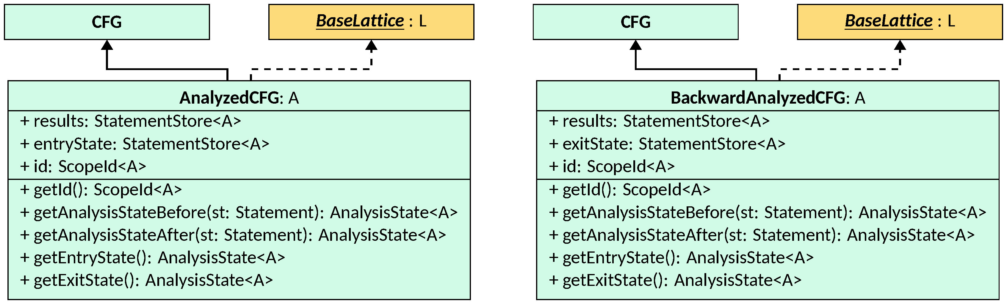
These are parametric to the type A extends AbstractLattice<A> that the results
(i.e., AnalysisState<A> instances) contain, and are subclasses of CFG
that contains methods to query the computed states
before or after a node, and of BaseLattice<AnalyzedCFG<A>> and
BaseLattice<BackwardAnalyzedCFG<A>>, respectively. Both classes provide
avenues for retrieving the entry or exit state of the whole CFG or of
individual nodes (i.e., Statement instances).
Each result is identified by a ScopeId, that will be
explained together with the interprocedural analysis interface.
For a list of fixpoint algorithms already implemented in LiSA, see the Configuration page.
Optimized fixpoints
Fixpoints can be optimized, as in they can be executed over the basic blocks of each CFG instead of the single nodes. When an optimized fixpoint is passed in the configuration, LiSA will compute the basic blocks of each CFG at the start of the analysis (see the CFG page for more details). Then, the fixpoints will proceed as if each basic block is a single node whose semantics is the composition of the semantics of the nodes it contains. This allows to skip both the traversal of the edges between nodes in the same basic block and the comparison of the results of each node, thus significantly reducing the time required to compute the fixpoint. Furthermore, after the fixpoint completes, all results are removed except for (i) the state after each widening point (e.g., loop guard) and (ii) the state after each call. This reduces memory consumption, and the results that have been forgotten can be recomputed with a single local fixpoint iteration. This process is called unwinding in LiSA.
All fixpoint implementations provided by LiSA have an optimized version:
OptimizedForwardAscendingFixpoint, OptimizedForwardDescendingGLBFixpoint,
OptimizedForwardDescendingNarrowingFixpoint, OptimizedBackwardAscendingFixpoint,
OptimizedBackwardDescendingGLBFixpoint, and OptimizedBackwardDescendingNarrowingFixpoint.
These can be passed in the configuration using the same options.
A common situation for static analyzers is to have visitors inspecting the
semantic results to issue warnings. In such a situation, the optimizations
performed by the above fixpoints would be nullified as unwinding is needed at
every program point that needs to be inspected. For this reason, as part of the
configuration, LiSA allows to select additional
instructions for which the results of fixpoints must be kept to avoid excessive
unwinding. The hotspots option is a predicate that, whenever it holds for a
node, forces the fixpoint to keep the results of that node even when an
optimized fixpoint is used. This allows to keep the results of nodes that are
relevant for the analysis, while still benefiting from the optimizations for the
rest of the nodes.
Results of optimized fixpoints are stored in OptimizedAnalyzedCFGs and
OptimizedBackwardAnalyzedCFGs, respectively:
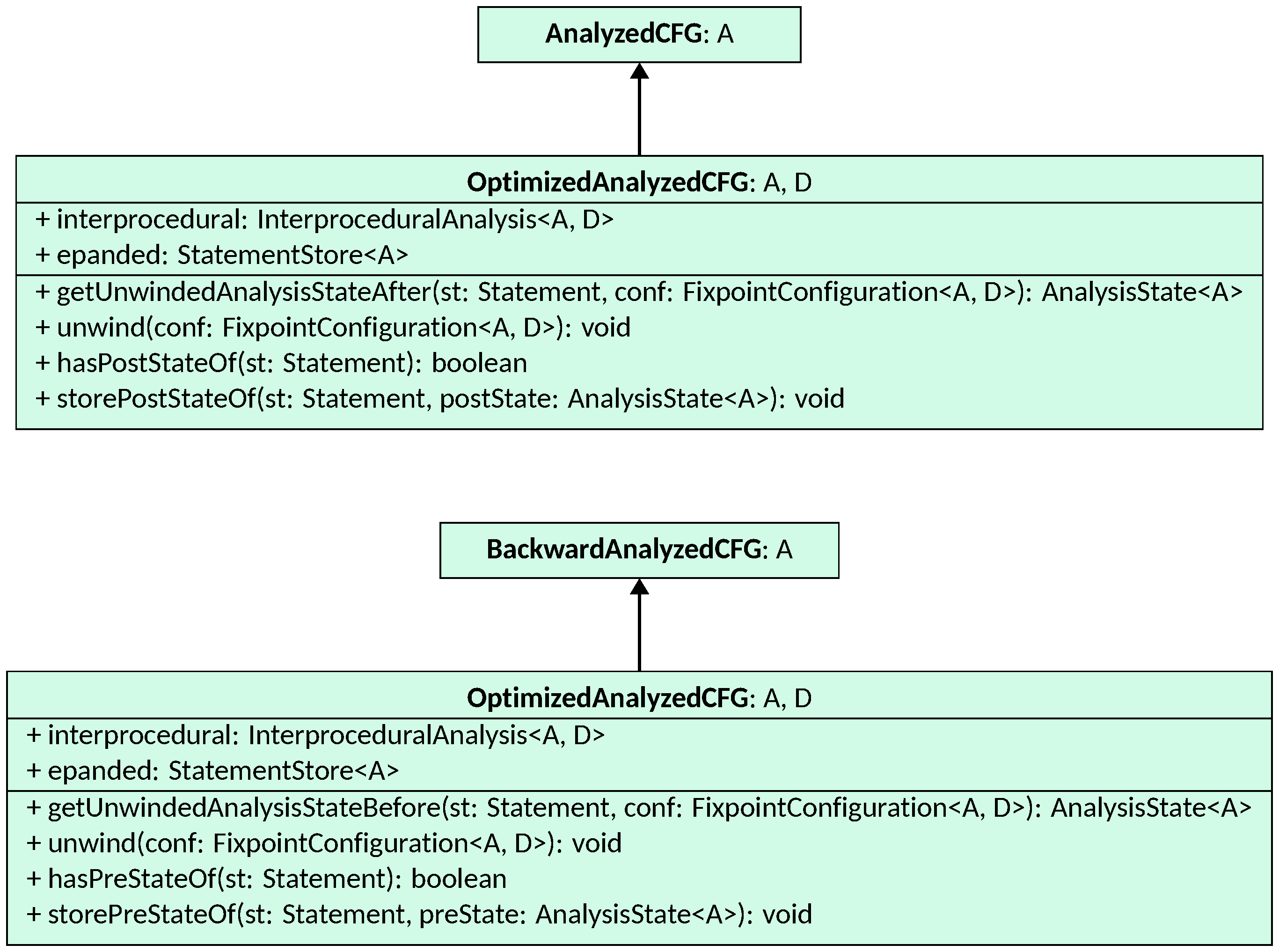
These inherit from AnalyzedCFG and BackwardAnalyzedCFG, respectively, and
add as type parameter the type D extends AbstractDomain<A> that the analysis
executes (necessary for performing unwinding). The main difference w.r.t. their
base classes is that they offer methods to unwind the results (unwind) or to
unwind only if necessary (getUnwindedAnalysisStateAfter/Before).
Prerequisites
The Fixpoint Configuration
Analysis options that are related to fixpoint executions are passed around
relevant methods through the FixpointConfiguration class, that mainly holds
values that have been passed in the main configuration:
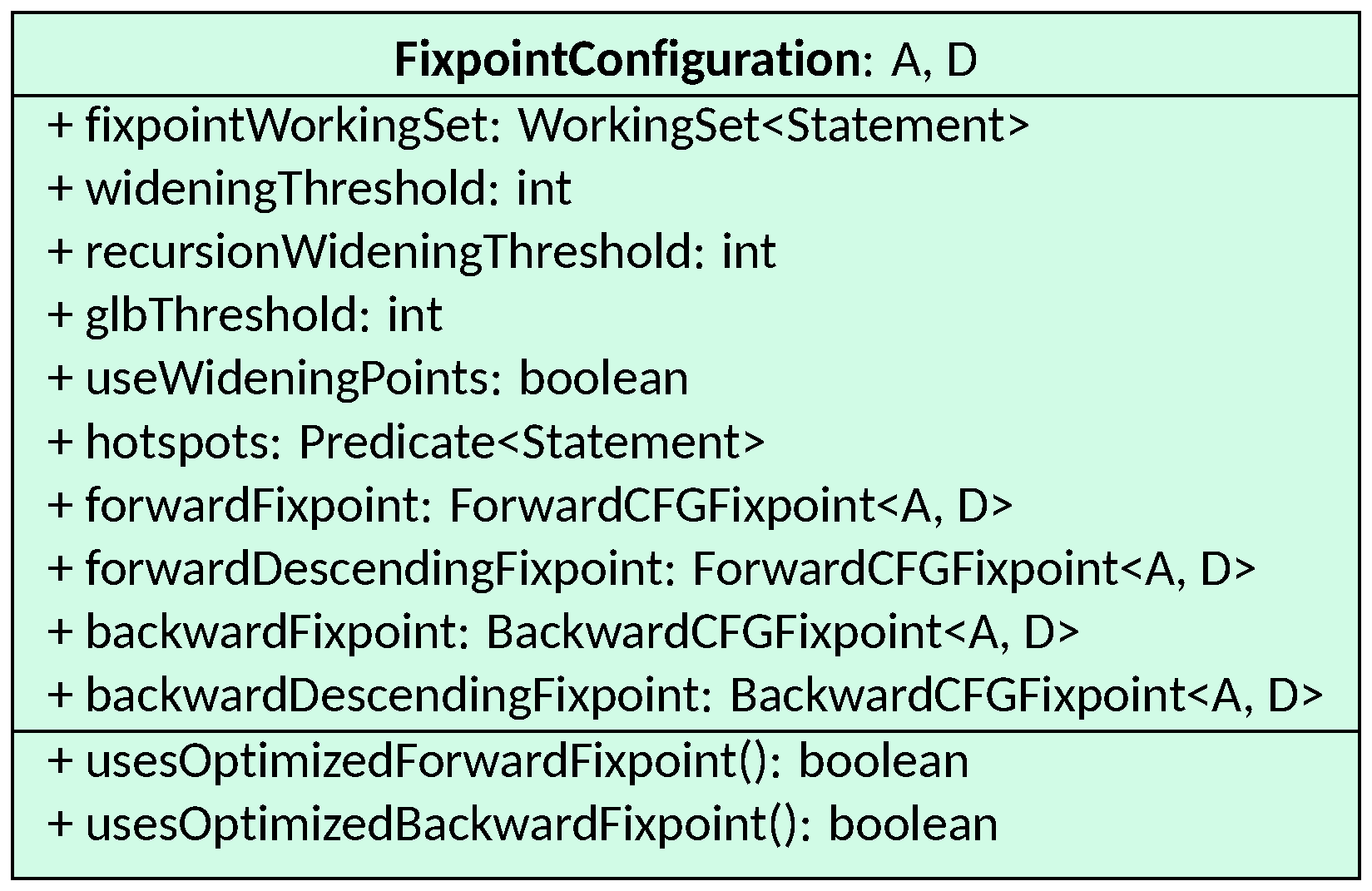
The configuration holds (i) the instance of WorkingSet to use in fixpoints,
that can be used to tune the order in which nodes are analyzed, (ii) several
thresholds for widening and glb applications inside fixpoints, (iii) the
instances of fixpoint algorithms selected for the analysis, (iv) whether or not
widening/narrowing should be applied only to widening points (useWideningPoints),
and (v) the predicate for selecting hotspots (hotspots). The two methods serve
as predicates to check if optimizations are enabled.
Scope Identifiers
A single CFG can be analyzed multiple times during the analysis, for instance
when its code is invoked at different call sites. If Interprocedural Analyses
want to distinguish between different invocations of the same CFG, they must
identify them by abstracting the concrete call stack. This is modeled in LiSA
with the ScopeId class:
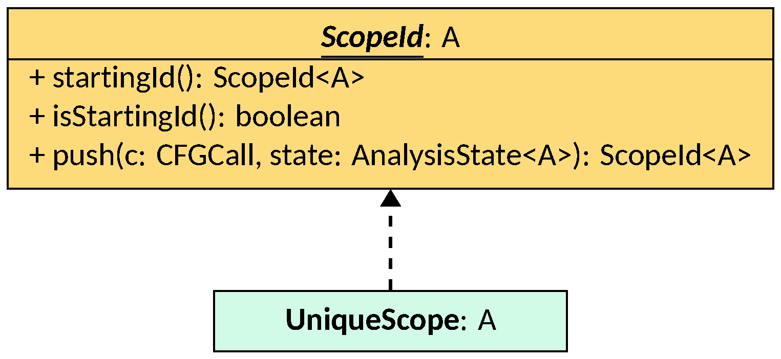
A ScopeId is parametric to the type A extends AbstractLattice<A> of the
states that the analysis computes. There is no particular structure required for
its instances: different analyses can abstract different parts of the call stack
(e.g., the call sites, the height of the stack, the states reaching each call
site, etc.). Each implementation must provide three methods:
startingId, that returns theScopeIdto use for the initial CFGs selected as entry points for the analysis;isStartingId, that checks if a givenScopeIdis a starting one;push, that returns a newScopeIdthat abstracts the call stack obtained by performing the given callc, reached with statestate, on the currentScopeId(i.e.,this).
In push the type of the parameter c is CFGCall. The Call hierarchy is
discussed in the Call Graph page,
but it is sufficient to know that it models calls that have been resolved and
whose targets are CFGs under analysis.
If analyses do not distinguish between different invocations of the same CFG,
they can use the UniqueScope class as ScopeId, that abstracts the whole call
stack as a single element. Results from different calls will thus be merged
together.
Handling Calls with no Targets
In LiSA, OpenCalls are calls that have been resolved, but no viable target
has been found inside the program under analysis (the Call hierarchy is
discussed in more depth in the Call Graph page).
The handling of such calls is independent of the Interprocedural Analysis:
regardless of the technique used to compute the results of calls, if no targets
are available, then no reasoning can be performed on the call.
To avoid reimplementation of Interprocedural Analyses that just differ in how
they handle OpenCalls, LiSA provides the OpenCallPolicy interface, that defines
the policy to apply when an OpenCall is encountered during the analysis:
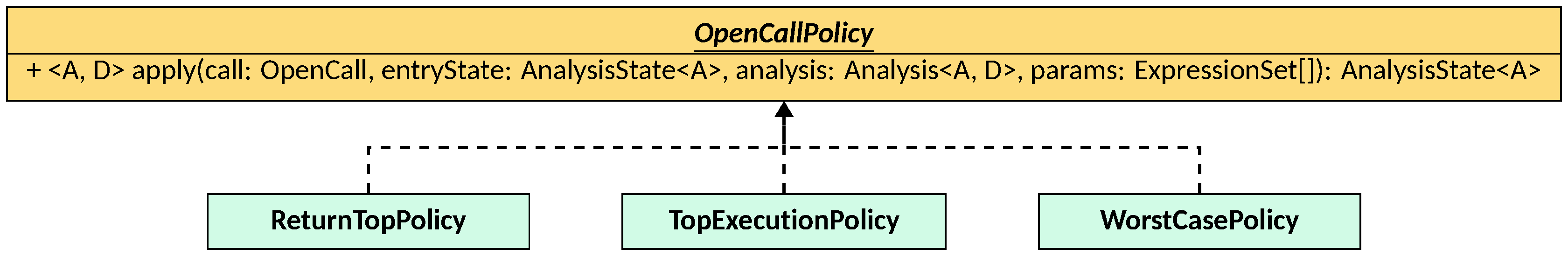
An OpenCallPolicy is simply a wrapper around the apply method, parametric on
the types A extends AbstractLattice<A> of states that the analysis computes
and D extends AbstractDomain<A> of the domain that the analysis executes,
that computes the effects of the OpenCall on a given state. The method has
access to all the semantic information (i.e., the entryState and the params
of the call), together with the call itself, to produce any sound (or
reasonable) result.
LiSA provides three base implementations of OpenCallPolicy:
WorstCasePolicy, that is the only fully sound policy, that returns the top element of the domain for any call, thus assuming that the open call can do anything to the program state and can raise any error;TopExecutionPolicy, that assumes that the call does not raise any errors, but can still tamper with the execution state in any way (in practice, this corresponds to setting the state’s normal execution to the top element of the domain while leaving the other continuations unchanged);ReturnTopPolicy, that assumes that the call does not raise any errors, cannot tamper with the execution state, but it has an unknown return value (in practice, this corresponds to returning the same state with aPushAnysymbolic expression as normal execution’s computed expression).
These are just commonly used policies, but users can implement their own policies. For a list of policies already implemented in LiSA, see the Configuration page.
Storing Fixpoint Results
All Interprocedural Analyses have to store the results of each CFG fixpoints for
later usage, e.g., for producing outputs
or executing semantic checks.
Storage is centralized in two classes, FixpointResults and CFGResults:
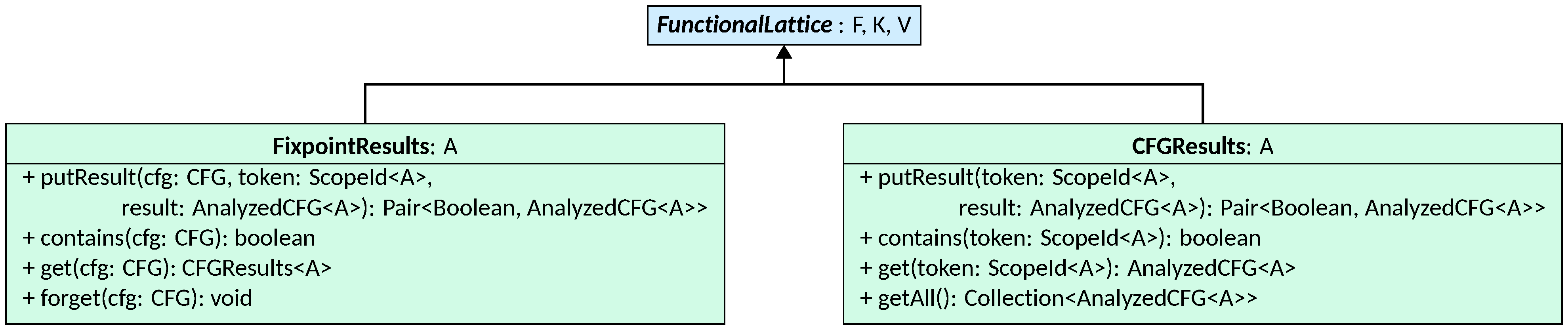
CFGResults, parametric on the type A extends AbstractLattice<A> of the states that the
analysis computes, is a function from ScopeIds to AnalyzedCFGs. It provides
avenues for querying if a result is present for the given token through
contains, and for retrieving the result through get. Instead, getAll
returns the flat collection of all values of the mapping, i.e., all the AnalyzedCFGs.
To store new results, putResult is provided. This method takes as parameters
the ScopeId to which the result belongs, and the AnalyzedCFG to store.
The method returns a pair of a boolean and an
AnalyzedCFG according to the following rules (where prev is the previous
result stored for token):
- if no
previs present, thentokenis mapped toresultand the method returns(false, result); - if
leq(prev, result), thentokenis mapped toresultand the method returns(true, result); - if
leq(result, prev), then the mapping is left unchanged and the method returns(false, prev); - if
prevandresultare not comparable, then the mapping is left unchanged and the method returns(true, lub(prev, result)).
The meaning of the returned pair is to be interpreted in terms of soundness: since the stored mapping must be an over-approximation for the given scope, one cannot simply store. Instead, the logic ensures that the result stored after the call is always the least precise one (i.e., the one that guarantees the over-approximation), and that is returned as second element of the pair for later usage by the Interprocedural Analysis. The boolean returned as first element is a flag that indicates whether the storage operation caused existing results to be invalidated, requiring the Interprocedural Analysis to reanalyze some CFGs.
FixpointResults, parametric on the type A extends AbstractLattice<A> of the states that the
analysis computes, lifts the mapping of CFGResults back to CFGs, so that
all results for a given CFG can be retrieved regardless of the ScopeId they belong to.
Note that FixpointResults’s putResult operates according to the same rules
of CFGResults’s putResult.
The Interprocedural Analysis Interface
The InterproceduralAnalysis interface defines all operations that an
Interprocedural Analysis must implement to be executed by LiSA:
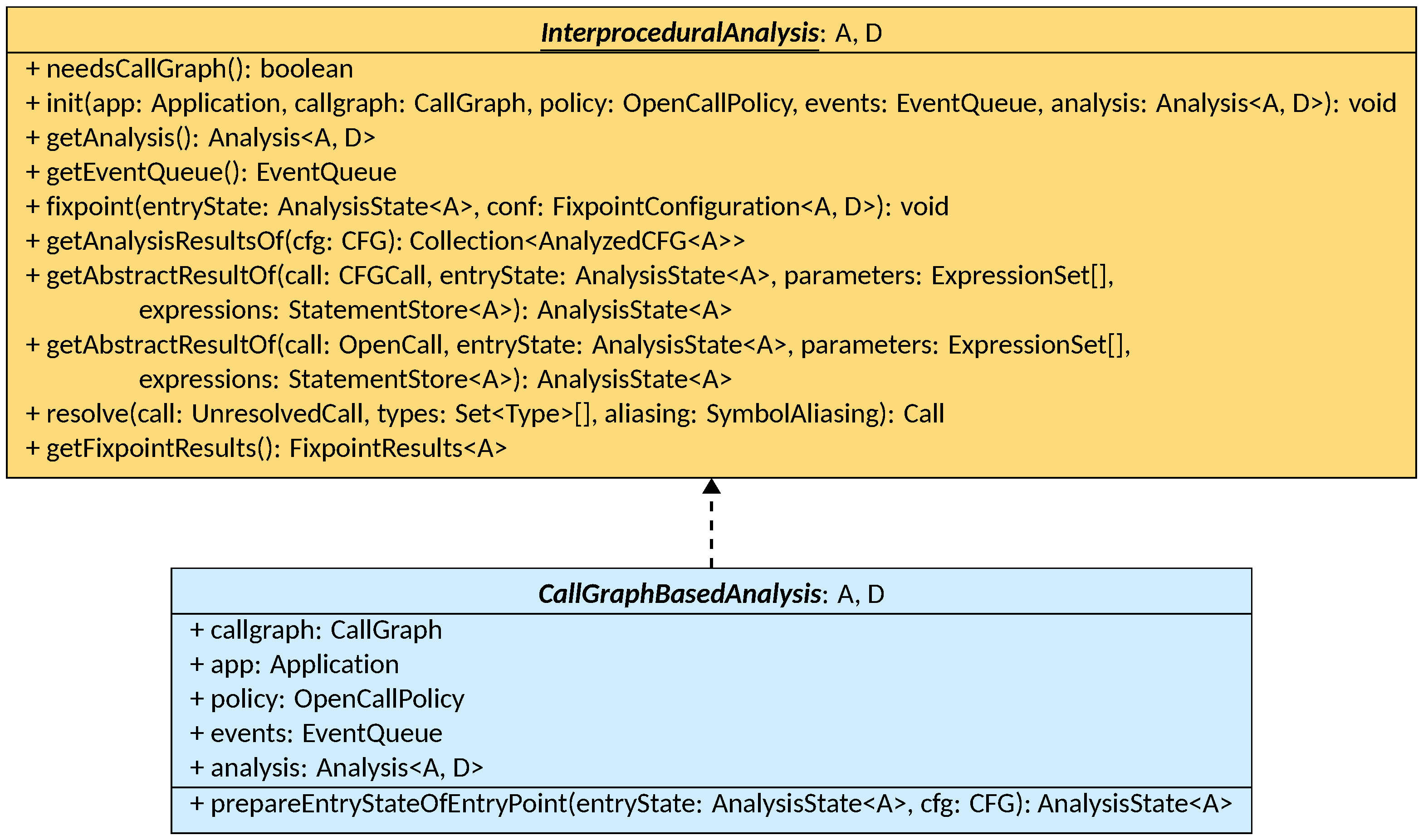
The analysis is initialized by LiSA by calling the init method, that passes
the analysis-specific configuration:
- the Application to analyze;
- the Call Graph to use for call resolution;
- the
OpenCallPolicyconfigured by the user; - the Event Queue to use for emitting events during the analysis;
- the
Analysisbuilt with theAbstractDomainconfigured by the user.
Note that the call graph is optional: the user might not select one for the
analysis. If the InterproceduralAnalysis implementation requires a call graph,
needsCallGraph must return true, and LiSA will throw an exception if no
call graph is provided. If needsCallGraph returns false, the call graph
parameter might be null. Furthermore, as noted in the
Event Queue page, the event
queue won’t be created if no listeners are registered for the analysis,
so the parameter might be null. Usages of the event queue should be
null-checked before emitting events.
The fixpoint method is the main entry point for the analysis, and is called
by LiSA to compute a program-wide fixpoint over all the code that has been
passed in the application. The method is passed an initial AnalysisState to
start the analysis from, and a FixpointConfiguration to use for fixpoint
executions. The method must proceed in starting the analysis by selecting
the CFGs to analyze as entry points, and executing a forward or backward
fixpoint over them. For reproducibility, it is highly advised that the order in
which entry points are analyzed is deterministic, e.g., by sorting them according
to their signature. The method must not return anything: during the analysis,
results of fixpoints must be stored in a FixpointResults instance, that is
returned by the getFixpointResults method. Invoking this method before
the analysis has been completed will return partial and possibly unsound
results. Results of individual CFGs can be obtained through the
getAnalysisResultsOf method, that returns a flattened view of the fixpoint
results for all ScopeIds of the given CFG.
For a list of interprocedural analyses already implemented in LiSA, see the Configuration page.
Handling Calls
The remaining three methods, namely resolve and the two getAbstractResultOf
overloads, are related to the handling of calls.
If the analysis is intraprocedural, as in it does not model calls from one CFG to another,
then resolve can return an OpenCall (i.e., a call that has been resolved,
but no viable target has been found inside the program under analysis —
see the Call hierarchy in the Call Graph page)
for any call, that will result in the invocation of the getAbstractResultOf
overload accepting the open call. Otherwise, the analysis should rely on the
CallGraph instance received in init to resolve calls through its own
resolve method, and return the resulting Call.
As discussed above, OpenCalls are handled according to the OpenCallPolicy
configured for the analysis: the getAbstractResultOf overload accepting an
OpenCall should delegate to the policy’s apply method to compute the result.
Instead, the getAbstractResultOf overload accepting a CFGCall
(i.e., a call that has been resolved and whose targets are CFGs under analysis —
see the Call hierarchy in the Call Graph page)
should:
- inform the
CallGraphthat the call is being executed by invoking theregisterCallmethod, so that it can be tracked in the graph’s structure; - update the current
ScopeIdif necessary by invoking thepushmethod; - compute the result of the call for each target independently by:
- using the program’s Scoping Logic to hide the caller’s variables behind the call site (see Scoped Objects for more details);
- using the program’s Assigning Strategy to assign the actual parameters of the call to the formal parameters of the callee;
- computing the result of invoking the target (e.g., by running a fixpoint over the target’s CFG or by accessing a previously computed result);
- using the program’s Scoping Logic to remove the callee’s variables and restore the caller’s ones;
- performing cleanup operations through
Analysis.transferThrowersandAnalysis.onCallReturn;
- joining the results of each target together.
This general workflow might need slight adaptations depending on the particular Interprocedural Analysis being implemented.
Note that return and throw statements will leave on the state’s
computedExpression a special Identifier (either a CFGReturn or a CFGThrow — see
the Identifiers page)
that will contain all Annotations
defined in the target CFG. This allows the propagation of invariants defined
through annotations from the callee to the caller.
Analyses based on Call Graphs
If an Interprocedural Analysis relies on a call graph, it is highly advised to
inherit from CallGraphBasedAnalysis. The class provides default
implementations for init, that stores all the parameters in the class’ fields,
resolve, that delegates to the call graph’s resolve method, getAbstractResultOf
for OpenCalls, that delegates to the OpenCallPolicy, and needsCallGraph,
that returns true. Moreover, it already implements the logic for creating
an entry state for the program’s entry points by assigning unknown values
to each parameter of the entry points.